Journal number 3 ∘ Lasha Kavtaradze ∘
INVESTIGATING SAVINGS-INVESTMENT GAP IN GEORGIA

Summary

Prior to the global financial crisis, Georgia faced high foreign investment inflows with expanded domestic credits and government expenditures. High inflation and a positive output gap were also the other two major issues that Georgia had to face with during this period. A combination of these shocks associated with a sizable negative savings-investment gap during the 2006-2008 periods. However, the negative savings-investment gap narrowed and reached to a historically low level of 5.8% by 2013.

In this paper, I investigate the driving factors that have determined the savings-investment gap in Georgia. I use the “Jacknife Model Averaging” Estimator to show private credit, GDP gap, FDI inflows, government expenditure and other indicators effects on the Georgian savings-investment gap. Effects of FX reserves and inflation on the savings-investment gap in Georgia constituted further findings of my study. While my analysis shows that the current account deficit supports the economic growth in the medium term. To achieve a sustainable growth path, Georgia must encourage savings, which is currently lower than its optimum level.

Keywords:Savings,Investment, Georgian Economy, Jacknife Model Averaging.

Jel Codes: E21, E22, E62, F32, F41.

 1. Introduction

Sustainable economic growth can be achieved only by increase in potential gross domestic product (GDP). The potential GDP per se is affected by capital, labor force and technological changes. While the latter component is very important, improvement in technology is feasible only in the long-run.  In the medium term, capital is an important driving factor of economic development. Hence, enabling stable flows of long-term capital (such as foreign direct investment) to countries with large investment needs must be a priority. Evidence shows that with greater levels of capital, not only does the output grow at a faster rate, but also the pace of technological improvement quickens; thus, providing a further catalyst for achieving sustainable economic growth.

The role assigned to investment in the process of economic growth is certainly relevant in growth theory and policy making. A major source of investment is savings. Hence, a linkage between savings and investment arise because “an increase a national saving has a substantial effect on the level of investment” (Feldstein and Baccetta, 1991).

Some studies (Barro 1991, Caselli, Esquirrel and Lefort 1995, Islam 1996) suggest that growth rate and investment (savings) co-move when there is a positive productivity shock. Taking the latter (productivity) as a constant, then one wonders if countries should increase investments and savings rates by accelerating the pace of their economic growth? Are there reinforcing effects between balanced savings-investment and growth? What are the main determinants of driving savings-investment gap? These are the questions that I will answer in this paper.

As various studies show, in the medium-term, for having 6-7 percent of economic growth an economy needs to maintain an investment level that is no less than 30 percent of GDP[1]. Investment is possible when total savings are sufficient. If savings rates are falling, a continued economic contraction is the possible result, with decreasing GDP and falling living standards.

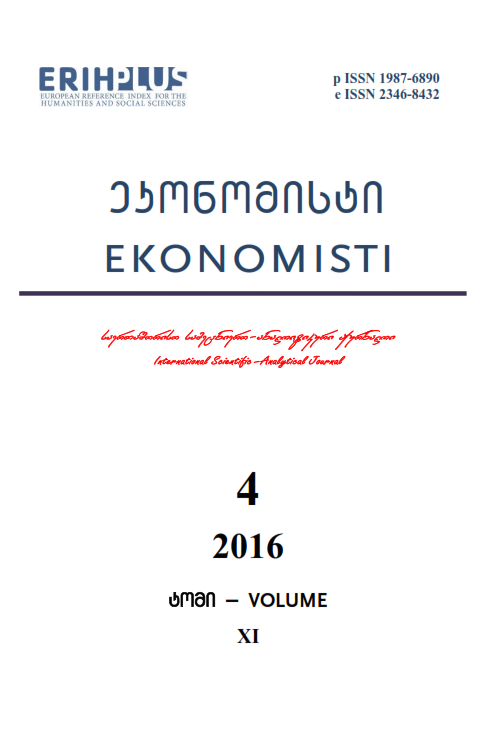
In some countries including Georgia, savings-investment imbalances had widened markedly in the years prior to the crisis (Figure 1). The savings-investment gap was relatively steady until 2005. The constant gap increased sharply when savings reduced drastically. However, the gap has started reducing since 2011, when both investments and savings bounced back. During the high savings-investment gap, the real growth rate of gross domestic product (GDP) ranged between 7-12 percent (with exception of 2008-2009), and the GDP growth slowed when the gap narrowed. This was mainly due to a higher decreasing speed of investment than that of savings. Regardless of a 25% investments of GDP ratio in 2013, economic growth slowed down (from 6.4% to 3.3%), enabling us to assume that Georgia did not have a strong basis for both economic growth and job creation.

Figure 1: Savings & Investments

 

     Source: The National Statistics Office of Georgia; Ministry of Finance of Georgia.

Facing the fact that, the Georgian economy is very sensitive to changing investment environment and is trapped in non-desired savings rate environment, a long-run high economic growth rate appears to be not its horizon. In the transition economies, including Georgia, high growth rate fixed when savings-investment gap was considerably high, more precisely, when the current account balance was reflected by a low level of national savings with respect to investment.

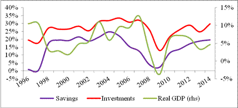
Since 1996 Georgia has been running both current account and fiscal deficits. The deficits narrowed during 1996-2004, but then reversed sharply in the periods of high economic growth (which mostly was driven by high inflows of foreign direct investments), and the CA deficit picked up at 22% of GDP in 2009 and the fiscal deficit - at 9.2% of GDP in 2009 (Figure 2).

Figure 2: The “Twin Deficit”

  Source: The National Bank of Georgia; Ministry of Finance of Georgia.

During the global financial crisis nominal exchange rate (GEL/US dollar) depreciated by 12.1%, and 6.7% in 2009 and 2010, respectively. This, in conjunction with lower domestic demand and reduction in FDI inflows led more than halved CA deficits (it reduced and reached at 10.6% in 2009 and 10.2% in 2010), however, sharply deteriorated fiscal deficits (9.2% in 2009 and 6.7% in 2010). Later on, in 2013, the CA deficits improved to its lowest at 6% of GDP.

Taking all the fact into account with additional features of the Georgian economy, investigating and understanding the determinants of savings-investment gap is pivotal from a policy perspective for Georgia[2]. The gap caused by a reduction in savings is likely to have more adverse consequences than the one caused by an investment boom that contributes to the future growth and a country’s ability to repay its (government) debt.            

Given the complex dynamics of the savings-investment, fiscal deficit, and current account balance, the main goal of this paper is to investigate the determinants of savings-investment gap in Georgia. This will require a special focus on those factors that are driving the current account balance and its dynamics with fiscal deficit.

2. The Model 

2.1. Identities

National accounts allow us to identify sources of investments by the following well-known identity:

S=I+X-IM+NFI+NTR (1)

where, S consists of private and government savings, I - investments (including government capital spending), X - exports, and IM – imports, NFI – net factor income from abroad, and NTR – net current transfers from abroad. Noting that X-IM+NFI+NTR is the account balance (CAB), then the aggregate public and private savings S is:

S=I+CAB (2) 

This shows that savings are the sum of investments and current account balance. Savings transform into investments or outflow abroad if the current account balance is positive:

I=S+CAD (3)

Where, Current account deficit = -current account balance (CAD = -CAB). Thus, investment is the sum of savings and current account deficit. This identity has an important conclusion: in countries, where income levels are low and therefore low propensity to savings, a main source of investment is foreign funds (current account deficit). In these countries, including Georgia, balancing the current account may cause a decrease in investments without any changes (increase) in domestic investments. Therefore, current account deficit for the developing countries is an “allowance” for economic growth. Certainly, in the medium-term, private saving is expected to grow along with an increase in economic growth and revenue gradually creates a room for investments to be funded domestically, which in turn brings the current account deficit down (or balancing).

On the other hand, for a developing country with positive current account balance (fewer investments than domestic savings), savings tends to outflow to other countries causing economic slowdown at home.

In the equation (3), savings are composed of the private sector and the public sector savings. The latter is the difference between government current revenues and expenditures (net operating balance). The government saving can be easily managed through the use of budgetary policy, but having impact on the private sector saving is a much more complicated task.

Other things being equal, an increase in government saving automatically increases the size of the investment, regardless of whether government capital expenses increase or not. Reduced current account deficit can be compensated by an increase in government saving. However, if the current account deficit (as a % of GDP) is sufficiently high, then this compensation cannot be achieved by (only) the fiscal policy.

Equation (3) can be rewritten as:

Ip+Ig=Sp+Sg+CAD (4)

Equation 4 shows that, if the government increases the capital expense with no changing in savings or current account deficits, this yields a non-increasing path for the total investment. In this case, the government investment crowds out the non-government investment, while the total investment capacity remains unchanged. In fact, built-in inefficiencies in the government capital expenditures may reduce speed of the economic growth. The gross investment level will grow if the government investment grows in accordance with the growth of government saving[3].

In Georgia, during 1996-2000, the government saving was negative, which led to reducing in total investment and slowed economic development. Since 2001, the government saving has been positive, but as shown in  Figure 3, a decrease in the investment level during the global crisis of 2008-2009, partially was related to the reduction of the government saving. One also should note that during the  2006-2009 periods, private saving was significantly reduced as well--the  increase in the current account deficit were neutralized by narrowing the private saving at the initial stage.

Figure 3: Decomposition of Savings

 

Source: Ministry of Finance of Georgia; the National Statistics office of Georgia.

In 2004-2008, a major source of growing investments was the current account deficit. In the absence of a decline in private saving, the economic growth would have been higher than what was the actual experience in Georgia.

Last year, sluggish economic growth was driven by decelerating of the total investment, which in turn was a reaction of the current account balance improvement.

As mentioned above, the target of economic growth (6-7 percent) is needed to achieve the 30% level of the investment to GDP. In Georgia, during the period of 2008-2013, the private saving to GDP was almost to 20%. One may assume that this will be maintained over the medium-term period. Calculations show that foreign debt stabilization is supported by 7.5% current account deficit to GDP ratio[4].  If we assume, in the medium-term, current account deficit will remain at the debt stabilizing level, then achieving the desired investment level for the economic growth requires having government savings of no less than 2.5% of GDP. If current account deficit remains at the 2013 level (5.8% of GDP), government saving can be no less than 4.0% of GDP. This implies that the budgetary policy has also an important impact on savings-investment decision.  However, in the case of increased current government spending, and a natural deviation from the optimum government saving level, there is no guarantee for achieving a sustainable economic growth path in the near future. 

2.2. Model Averaging

To analyze determinants/factors of current account balance in Georgia, I use model averaging to estimate unknown parameters of the model.

The two most favored approaches to treat model uncertainty are model selection and model averaging, while both Bayesian and non-Bayesian methods have been proposed. By the nature of the average, model averaging is more robust than model selection, as the averaging estimator considers the uncertainty across different models together with the model bias from each candidate model (Hansen, 2007; Haddad and Nedeljkovic, 2012).

In this paper, I use a “Jackknife Model Averaging” (JMA) estimator for non-nested and heteroscedastic models (B.E.Hansen, J.S.Racine, 2012) which selects the weights by minimizing a cross validation criterion. In models that are linear in the parameters the cross-validation criterion is a simple quadratic function of the weights, so the solution is found through a standard application of numerical quadratic programming.

Thus, using the JMA, I am going to estimate the following simple regression[5]:

Y_t = X_tβ + ε_t  (5)

E(ε_t|X_t) = 0

E(ε²_t|X_t) = σ²(X_t)

Where, Y_t is the current account to GDP ratio (dependent variable), while X_t is the d-dimensional vector of explanatory variables,  is random error term that is allowed to be heteroskedastic. No assumption on the distribution of the error term is imposed.

In this paper, I use some of explanatory variables measured by applying different approaches, while following variety possible variations suggested by Cusolito and Nedeljkovich (2013). For instance, output gap employed in this paper is measured by using multivariate filter, such as a Kalman filter augmented by Phillips curve, instead of Hodrick-Prescott filtering method. Also, the paper exploited cyclically adjusted government expenses (elasticity of expenses with respect to the output gap is 0.2; however, for the robustness check I used a zero elasticity too) instead of a simple government expenditures ratio to GDP, or a budget balance ratio to GDP.

Let Ω be the number of models where each model m=1....Ω , represents a particular subset of the explanatory variables X_tm whose dimension is smaller than d. The OLS parameter estimate for the m^th model is, simply:

The averaging estimator for the full regression model is:

 

Where, the weights,W_m, are assumed to be non-negative and sum up to one. The JMA estimator selects the weights by minimizing a leave-one-out cross-validation criterion. Hansen and Racine (2012) showed that the average squared error of the JMA estimator asymptotically attains the lowest average squared error among all feasible weight vectors.

3. Data

To estimate the equation (1) annual data is used over 1996-2013. The dependent variable is the current account balance to GDP ratio. The set of explanatory variables[6] includes: real GDP per capita (PPP); GDP gap[7]; and real exchange rate (REER).  I also add oil prices (in log change) instead of terms of trade (TOT) because: in a highly dollarized economy (60%[8]) such as Georgia, the REER not only captures TOT effects, but also balance sheet effects that may arise after REER shocks. Moreover, in an oil importing country like Georgia, oil prices affect the CA balance in its own right. Other explanatory variables studied in the paper are: trade openness; net international investment position (NIIP); cyclically adjusted government expenditure (% of GDP); foreign reserves (% of GDP); fertility rate; foreign direct investment (FDI) (% of GDP); relative GDP growth; credit of private sector (% of GDP) and moving average inflation volatility.

The sources of the data (Georgian Data set[9]) used in this paper are:  The National Statistics Office of Georgia (GEOSTAT), the National Bank of Georgia (NBG), the Ministry of Finance of Georgia (MoF), the International Monetary Fund (IMF) and the World Economic Outlook (2013).

3. Estimation Results

The predicted current account balance (CAB) obtained by using the JMA estimator is shown below (Figure 4).

Figure 4: Estimation Results of CAB for Georgia

Source: Author’s calculation.

As we see, the weighted average result of all possible models performs nicely. Detail results – impacts of various macro-fiscal variables on the CAB – are presented below in the table. This table reports the standardized estimates, because exogenous variables captured in the model are measured in different units of measurement and express the change in the dependent variable in standard deviations, induced by a change in one standard deviation of the explanatory variable. All estimated coefficients are statistically significant and have expected signs[10] (see appendix for the detail description of exogenous variables captured in the JMA model)[11].

         *** Significant at the 1% level; ** significant at the 5% level; *significant at the 10% level.

    Standard errors are in parentheses;   

    Source: Author’s calculation.

 Evidence from the empirical literatures (Sachs 1981; Obstfeld and Rogoff, 1995,1996; Ghosh 1995; Rasin 1995; Glick and Rogoff 1995), measuring influences of various economic variables on current account balance is highly depended on countries’ specific factors and more often the impact is ambiguous.  As we see from the Table 1, the most important variables in determining of the current account deficit in Georgia are: the foreign direct investment (FDI), the private credit, the stock of foreign exchange reserves, the government expenditure, the relative GDP growth to its top traders and the output gap.

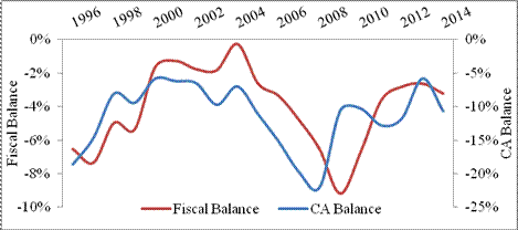
The coefficient of the output gap is constructed as the difference between actual and potential output estimated by using Kalman filter augmented by Philips curve. An increase in the output gap signals a boom in demand beyond supply capacity, which is associated with a reduction in saving. Therefore, one would expect that all other things equal, an increase in the output gap leads to a decrease in the CA Balance (or an increase in the deficit). The expected coefficient in the CA determinants regression, that captures the marginal change in the CA balance induced by a marginal change in the output gap is negative and statistically significant (-0.11). In fact, when GDP gap (Figure 5.) experienced a sharp increase from 2006 until the third quarter of 2008 (reached at its pick 6.1% in the third quarter on 2007) the CA deficit widened drastically (19.6% in 2007 and 22% in 2008).  It should be noted that, during these periods access to private credits (mostly from private banks) became much easier and its contribution to the national economy (in stock) increased by 5-7% as of GDP in 2007-2008. The fact that credit expansion boosts demand has a negative pressure on savings, which in turn deteriorates current account balance. According to our estimation, marginal impact of private credit changes to CA balance is negative and sizeable (-0.36). 

Figure 5: Output Gap in Georgia

  

Source: Author’s calculation.

In a small open economy country such as Georgia foreign investments are of paramount importance. Accumulating foreign reserves may have positive or negative effects on the CA balance depending on the FX role on the exchange rate (prevention of appreciation or depreciation). In Georgia, the FX sharply increased in 2007 and influenced on the currency, however, the monetary authority prevented its apparent appreciation. Therefore, as the model estimates shows, the FX reveals a positive effect to detain further widening of the CA deficit. In contrast with the FX, the foreign direct investment (FDI) displays negative effect on the CA balance (with highest standardized coefficient: -0.49), which can be explained by the fact that in Georgia major parts of FDI go to the non-tradable sectors[12] and it is mostly absorbed by purchasing imported goods.  As for the government expenditures, if it raises then demand increases that will be in part satisfied by additional imports (Ahmed 1996). The marginal negative effect (-0.16) of the government expenditure explains the CA deficit took place during 2005-2008, when fiscal deficit increased from -0.3% in 2004 to -2.6% in 2005 and reached at -6.5% in 2008.  

Apart from other small factors (indicated by their estimated negligible impacts), the above analysis provides a framework for taking into account the important factors that deserve serious consideration in the policy making process in the country. 

5. Conclusion and Policy Recommendation

In this policy paper, I investigated the determinants of the savings-investment gap in Georgia. Analysis shows, that the current account deficit for Georgia behaves as an “allowance” for the economic growth in the short- and medium terms. However, the current account balance creates significant uncertainty in the economy as well. Analysis shows that it is important that the government increases public investment in accordance with the public saving.

In Georgia savings and investment level are not sufficient for sustainable economic development, and when the CA deficit is caused by low saving, this poses uncertainty and risks in the allocation of resources.

Financial sector, which can play an intermediation role in boosting growth, in Georgia had been characterized as an instable sector until 2005, because of lack of confidence, weak institutions and infrastructure, unhealthy competition, and some regulatory restrictions (IMF country report, 2006).  According to the theory, such a feature of the financial system interferes to mobilizing and pooling savings. But in Georgia, when the financial system development has become feasible since 2005, the level of national savings declined, while public saving remained unchanged until the global financial crisis (2008). Such a behavior of the society after the revival of the financial system was revealed because of too easy access to the banking credit, and people, instead of making savings, started purchasing houses, other properties, consume more good and service. Thus, accessing of the financial resource has opened room for more consumption by reducing private saving level and caused deterioration in the CAB, which is found in my analysis by revealing high impact of the private credit (-0.36) on the savings-investment gap in Georgia.

The savings-investment gap in Georgia also is highly explained by the FDI, the government expenses, the FX reserves factors and the output gap.

Deterioration of the Georgian CA balance in the 2006-2008 periods was mainly due to a positive GDP gap, sharp increases in the private credit, higher government expenditures, high FDI, and high net foreign liabilities. 

Analysis shows that, for Georgia, it is more important to keep inflation volatility at minimum than focusing on the exchange rate stabilization. This is mainly due to the observation that the former (inflation volatility) has higher negative effect on the CAB than the latter (exchange rate fluctuation).

The finding that there is not sufficient savings in the Georgian economy is used as the preludes to discussing the possible scenarios for improve savings in Georgia.  Lack of an appropriate array of financial instruments hinders incentive and ability to save in Georgia.   Thus, creation of financial instruments in must be considered as an important step towards improving long-term savings in Georgia.

This paper also recommends further promotion of strategies that would encourage foreign investments into the tradable sector (manufacturing, agriculture, mining, retail, hotels and restaurants), since tradable sector is associated with higher exports.

Given the important role of government savings in influencing CAB, the government should maintain a minimum level of government savings is needed to stabilize the government debt and achieve moderate growth rate (but unsustainable). However, achieving a sustainable economic growth path needs high level of savings and investment.

And lastly, high current account deficit not only in Georgia, but also in other transition countries will remain the status of the “allowance” for the growth only in a case of neglecting external shocks. 

 6. References 

1. Apoteker, Th. And Kassay, A. (2014), “Currency and Current Account Rebalancing in Indonesia”, OECD Workshop, Paris.
2. Blanchard, O. (2007), “Current Account Deficits in Rich Countries”, IMF Staff Papers, Vol. 54.
3. Calderon, A., Chong, A. and Zanforlin, L. (2001), “Are African Current Account Deficit Different? Stylized Facts, Transitory Shocks, and Decomposition Analysis” IMF Working Paper.
4. Chinn, M.D., (2005), “Current Account Balances, Financial Development and Institutions: Assaying the World “Savings Glut” “, Working Paper 11761, Cambridge MA.
5. Choi, H. and Mark, N.C. (2009), “Trending Current Accounts”.
6. Calderon, A. Chong, A. and Loayza, N. (2002), “Determinants of Current Account Deficits in Developing Countries.” Policy Research Working Paper.
7. Carroll, C.D and D.N. Weil (1994), “Saving and Growth: A Reinterpretation”. Carnegie-Rocherster Conference Series on Public Policy.
8. Chinn, M.  and E. Prasad (2003), “Medium-term Determinants of Current Accounts in Industrial and Developing Countries: an Empirical Exploration”. Journal of International Economics.
9. Cusolito, A. and M. Nedeljkovic (2013), “Toolkit for the Analysis of Current Account Imbalances”, International Trade Department, World Bank, DC.
10. Debelle, G. and H. Faruque (1996), “What Determines the Current Account? A Cross-Sectional and Panel Approach”. IMF working Paper No. 58. IMF, Washington, DC.
11. Feldstein, M. and Bacchetta, Ph. (1991), “National Saving and International Investment”, National Berau of Economic Research.
12. Ghosh, A. and Ramakrishnan, U. (2014), “Current Account Deficits: Is There A Problem”, IMF.
13. Gruber, J.W., and S. B. Kamin (2007), “Explaining the Global Pattern of Current Account Imbalances”, Journal of International Money and Finance.
14. Hansen, B., and Racine, J. (2012), “Jackknife Model Averaging”. Journal of Econometrics.
15. Hermann, S. and Jochem, A. (2005), “Determinants of Current Account Developments in the Central and East European EU Member States – Consequences for the Enlargement of the EU Area”, Discussion Paper, Series 1: Economic Studies, No 32.
16. Hochreiter, E. and Gylfason, Th. (2008), “Growing Apart? A Tale of Two Republics: Estonia and Georgia”, IMF Working Paper, 235.
17. Kinoshita, Y. (2011), “Sectoral Composition of FDI and External Vulnerability in Easter Europe”, IMF Working Paper, 4.
18. Kwiatkowski, D., P.C. S. Phillips, P. Schmidt, and Y. Shin (1992),  “Testing the Null Hypothesis of Stationarity against the Alternative of a Unit Root” Journal of Econometrics.
19. Milesi-Ferretti, G.M. and A. Razin (1996), “Sustainability of Persistent Current Account Deficits”, NBER Working Paper 5467, National Bureau of Economic Research.
20. Obstfeld, M. and K. Rogoff (1996), “Foundations of International Macroeconomics”, Cambridge, MA: MIT Press.
21. Rangazas, P. and Mourmouras, A. (2008), “Fiscal Policy and Economic Development”, IMF Working Paper 155.
22. Reyes, J.D. and G. Varela (2013), “Georgia: Trade Competitiveness Diagnostic”, International Trade Department, PREM, Mimeo, Washington, DC.

Appendix

Unit Root Test on Stationarity

---